The bio package
Welcome to bio
bio is a bioinformatics toy to play with.
Like LEGO pieces that match one another bio aims to provide you with commands that naturally fit together and let you express your intent with short, explicit and simple commands. It is a project in an exploratory phase, we’d welcome input and suggestions on what it should grow up into.
If you’ve ever done bioinformatics you know how even seemingly straightforward tasks often require multiple steps, searching the web, reading documentation, clicking around various websites that all together can slow down your progress.
Time and again, I found myself not pursuing ideas because getting to the fun part was too tedious. The bio package was designed to solve that tedium by making bioinformatics explorations more enjoyable. The software lets users quickly answer questions such as:
- How do I download data by an accession number?
bio fetch NC_045512 > genome.gb - How do I view the sequence annotation of the data?
bio gff genome.gb - How do I get the coding sequence for a specific gene?
bio fasta --gene S genome.gb - What is the taxid for SARS-COV-2?
bio taxon sars2 - What is the lineage of SARS-COV-2?
bio taxon 2697049 --lineage - At what date were viral samples collected?
bio data 2697049 | head - What is a microsatellite?
bio explain microsatellite - What genes match the word
HBB?bio search HBB --species human
bio combines data from different sources: GenBank,Ensembl,Gene Ontology,Sequence Ontology,
NCBI Taxonomy and provides an unified, consistent interface.
The software is also used to demonstrate and teach bioinformatics and is the companion software to the Biostar Handbook.
Quick start
Install bio:
pip install bio --upgradeCode and info
- Source code: https://github.com/ialbert/bio
- Documentation: https://www.bioinfo.help
- Report errors: https://github.com/ialbert/bio/issues
- Discussion board (new): https://github.com/ialbert/bio/discussions
Usage examples
Suppose we found the accession number to data of interest: NC_045512 representing the Wuhan-Hu-1 isolate of the coronavirus and
MN996532 that stores information on the most similar bat coronavirus. We would like to investigate the differences in the S protein betweeen the two organisms. Here is how you could do it with bio:
Fetch data
bio fetch MN996532 NC_045512 > genomes.gbExtract sequences of interest
Look at the first 10 bases for the coding sequence of gene S:
bio fasta genomes.gb --end 10 --gene S | headprints:
>YP_009724390.1 CDS gene S, surface glycoprotein [1:10]
ATGTTTGTTT
>QHU36824.1 CDS gene S, surface glycoprotein [1:10]
ATGTTTGTTT
Align sequences
Let’s align the protein sequences for the S gene
cat genomes.gb | bio fasta --gene S --protein | bio align | headprints:
# PEP: YP_009724390.1 (1,273) vs QHR63300.2 (1,269) score=6541.0
# Alignment: length=1273 ident=1240/1273(97.4%) mis=29 del=4 ins=0 gap=4
# Parameters: matrix=BLOSUM62 gap-open=11 gap-extend=1

MFVFLVLLPLVSSQCVNLTTRTQLPPAYTNSFTRGVYYPDKVFRSSVLHSTQDLFLPFFSNVTWFHAIHVSGTNGTKRFDN
|||||||||||||||||||||||||||||||.|||||||||||||||||.|||||||||||||||||||||||||.||||| 81
MFVFLVLLPLVSSQCVNLTTRTQLPPAYTNSSTRGVYYPDKVFRSSVLHLTQDLFLPFFSNVTWFHAIHVSGTNGIKRFDN
Show alignment as mutations
Pairwise alignments can be overly verbose, let’s look at mutations alone:
cat genomes.gb | bio fasta --gene S --protein | bio align --mut | tailprints the type and variant at each location:
Y493Q   SNP     493     Y       Q
R494S   SNP     494     R       S
Y498Q   SNP     498     Y       Q
D501N   SNP     501     D       N
H505Y   SNP     505     H       Y
N519H   SNP     519     N       H
A604T   SNP     604     A       T
S680SPRRA       INS     680     S       SPRRA
S1121N  SNP     1121    S       N
I1224V  SNP     1224    I       V
It shows that at position 680 the coronavirus has a four aminoacid insertion PRRA, the so called furin-cleavage.
Visualize the genome data
Convert to GFF
bio gff genomes.gb | headprints:
##gff-version 3
MN996532.2      .       gene    266     21552   .       +       .       ID=1;Name=orf1ab;Parent=orf1ab;color=#cb7a77
MN996532.2      .       CDS     266     13465   .       +       .       ID=2;Name=QHR63299.2;Parent=QHR63299.2
MN996532.2      .       CDS     13465   21552   .       +       .       ID=3;Name=QHR63299.2;Parent=QHR63299.2
MN996532.2      .       gene    21560   25369   .       +       .       ID=4;Name=S;Parent=S;color=#cb7a77
MN996532.2      .       CDS     21560   25369   .       +       .       ID=5;Name=QHR63300.2;Parent=QHR63300.2
Load and view the resulting files in IGV
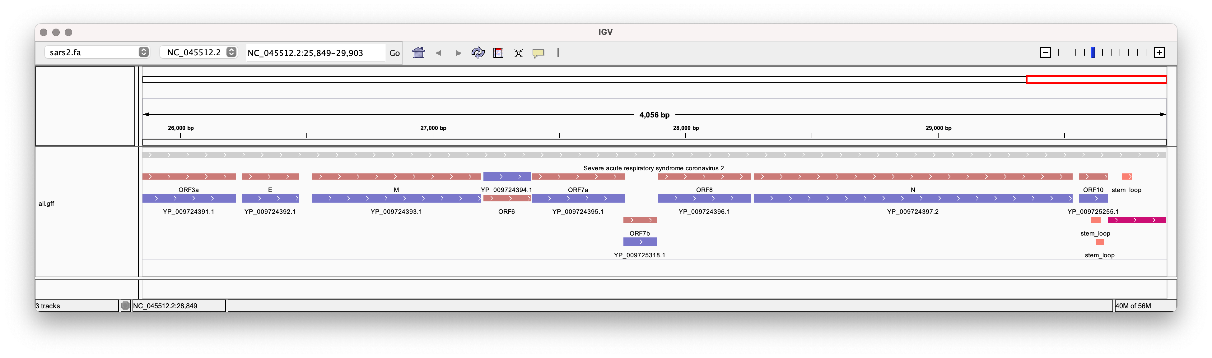
Among the many useful features, bio is also able to generate informative gene models from a GenBank file.
Where to go next
Look at the sidebar for detailed documentation on additional commands that bio supports.